A Completely Unnecessary Quantitative Investigation of the Washington Dating Market
My wife told me a story recently that presented itself as an ordinary conversation about dating. It should have remained one. Instead, I made the mistake of thinking about it mathematically.
Imagine a woman living in the Washington metropolitan area. She is Black, a physician, professionally established, financially secure, educated, and old enough to have accumulated both standards and evidence supporting them. She knows broadly what she wants in a partner. He must be Black. He should be in good physical shape. He must be employed, preferably in an established profession. He must love children. He should be respectful, socially intelligent, intellectually curious and, because apparently we are asking for everything now, fun.
Preferably, she says, he would be another doctor.
At first glance, none of this sounds particularly unreasonable. Washington is full of successful Black people. The metropolitan area has one of the largest Black populations in the country and an unusually professional labor force. Hospitals, universities, federal agencies, military installations, law firms, technology companies, consulting firms, financial institutions and an astonishing number of organizations containing the words strategic, global or institute employ armies of credentialed adults. On any given weekday, you can walk three blocks downtown and encounter enough graduate degrees to destabilize a developing economy.
Surely her man is somewhere around here.
But “somewhere around here” is not a probability.
And that is where the trouble begins.
The Patient Presents With No Husband
Let us approach the problem properly.
The first question is not whether our hypothetical woman will find a husband. Science cannot tolerate that level of imprecision. We must first establish the population at risk.
Washington, DC itself is too restrictive a geographic unit. Nobody sensible stops dating someone because he lives across an invisible municipal boundary in Silver Spring, Prince George’s County or Arlington. The relevant market is the greater Washington metropolitan area: the District and the surrounding Maryland and Virginia communities from which people routinely commute, socialize, date, marry and complain about traffic.
The Washington metropolitan area contains more than six million people. Roughly one and a half million identify as Black alone. Already, things look promising.
But our protagonist does not want to marry one and a half million people.
She wants one man.
So we begin filtering.
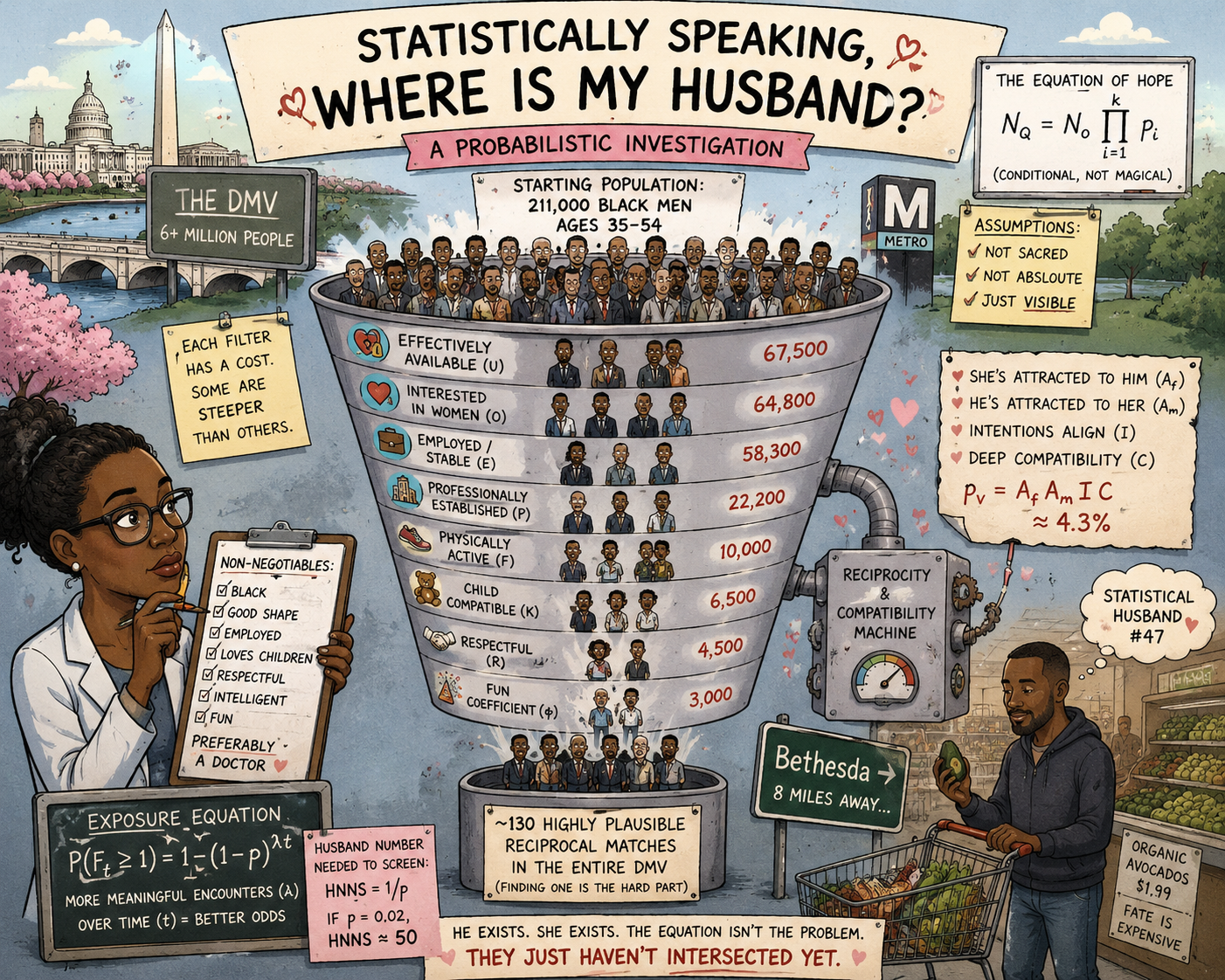
Suppose we establish an acceptable age range of 35 to 54. Using the region’s demographic structure to estimate the Black male population within that band gives us an initial working universe on the order of 211,000 men.
Call this population N₀.
At its simplest, our problem looks like this:
N_Q = N₀ × ∏ᵢ₌₁ᵏ pᵢ
where N_Q is the estimated number of qualifying men and each pᵢ represents the proportion surviving one additional requirement.
This is the equation that launches a thousand terrible internet articles.
The problem is that simply multiplying percentages assumes, implicitly or explicitly, that our filters can be treated independently. They cannot. Age relates to marriage. Education relates to occupation. Income relates to geography. Professional status may relate to physical activity. Parenthood relates to age and marital history. The probability that a 42-year-old Black physician is married is not necessarily the same as the probability that a randomly selected 42-year-old American man is married.
A more defensible formulation therefore uses conditional probabilities:
N_Q = N₀
× P(U | A, B)
× P(O | U, A, B)
× P(E | O, U, A, B)
× P(P | E, O, U, A, B)
× P(F | P, E, …)
× P(K | F, P, …)
× P(R | K, F, …)
× P(φ | R, K, …)
Here A represents age eligibility, B the Black male population, U romantic availability, O compatible sexual orientation, E employment and economic stability, P professional status, F fitness, K compatibility with children, R respectfulness, and φ what we shall eventually and irresponsibly call the Fun Coefficient.
The distinction matters. This is not a bag of independent percentages. It is a funnel of increasingly conditional probabilities.
With approximately 211,000 Black men in our working age band, however, our protagonist should initially feel optimistic. There are enough candidates to fill Capital One Arena roughly ten times.
If she cannot find one suitable person among them, surely something extraordinary must be happening.
Something extraordinary is happening.
They are human beings.
Unfortunately, He Must Be Available
The first major error in amateur dating mathematics is counting every unmarried-looking person as available.
A man may be married. He may have a girlfriend. He may have two girlfriends, neither of whom knows she is participating in a longitudinal study. He may be divorced but have no intention of dating seriously until 2031. He may describe himself as “separated,” a marital category whose precise meaning occasionally depends upon whether his wife is within earshot.
He may technically be single while maintaining a relationship sufficiently complicated that the Centers for Disease Control would classify further contact as an exposure event.
Regional marital statistics give us a useful starting point, but “not married” is not the same as “available.” Never married does not mean unattached. Divorced does not mean ready. Widowed does not mean looking. A proper model therefore needs an effective availability parameter rather than simply subtracting married men.
Let:
U = P(effectively romantically available)
For the baseline model, suppose:
U = 0.32
with a plausible scenario range of:
0.25 ≤ U ≤ 0.40
The 0.32 is not a discovered law of Washington romance. It is a modeling parameter informed by marital-status data and then adjusted downward to recognize that some legally unmarried men are nevertheless partnered, unavailable or uninterested in dating. The 0.25–0.40 interval is likewise not a formal 95-percent confidence interval. It is a scenario range: a deliberately visible statement that reasonable assumptions could move the parameter in either direction.
Under the baseline:
211,000 × 0.32 ≈ 67,500
We have eliminated roughly 143,500 candidates before asking whether anyone has a job.
This is our first important discovery.
The greatest threat to the Washington dating pool may not be women’s standards.
It may be other women.
Orientation Must Regrettably Be Considered
Next, our hypothetical physician is looking for a man interested in women.
Most men qualify. Some do not. Bisexual men remain in the eligible population because, contrary to some extraordinarily bad internet mathematics, bisexuality does not render a man incapable of dating a woman.
Let the orientation-compatibility parameter be O. A reasonable baseline might be:
O = 0.96
with:
0.93 ≤ O ≤ 0.98
This parameter has a relatively narrow range because national sexual-orientation data give us a much stronger empirical foundation than we will have for concepts such as “fun.”
Our approximately 67,500 candidates become about 64,800.
No crisis yet.
The Employment Department Arrives
Our woman requires that her prospective partner be employed.
Reasonable.
We can debate whether someone between positions counts, whether entrepreneurship without revenue constitutes employment, or whether a man who identifies himself as CEO of a company whose headquarters are his mother’s basement has satisfied the requirement. For the sake of civilization, let us define this criterion as genuine employment or demonstrable economic stability.
For prime-working-age candidates, suppose:
E = 0.90
and test:
0.85 ≤ E ≤ 0.95
The baseline is informed by prime-age employment patterns but remains a model assumption because the precise intersection we need—Black, male, 35–54, available, Washington metropolitan area—is not neatly delivered by one government table.
Under the baseline:
64,800 × 0.90 ≈ 58,300
Still healthy.
Then she adds:
“Preferably a professional.”
Ah.
We need another meeting.
The Professional Problem
Washington is unusually favorable here. The region is stuffed with physicians, lawyers, engineers, military officers, federal officials, professors, scientists, technology specialists, consultants, managers and policy professionals. If a woman insists on professional employment, Washington is probably one of the better American cities in which to make that demand.
But “professional” still carries a substantial Dating Pool Tax.
Suppose we define professionally established broadly enough to include medicine, law, engineering, technology, science, academia, management, finance, senior government work, established entrepreneurship and comparable occupations. For the first model:
P = 0.38
with:
0.25 ≤ P ≤ 0.50
That range is deliberately wide. “Professional” is partly definitional. A model that includes only physicians, lawyers and executives will produce a radically different result from one that includes senior civil servants, engineers, teachers, entrepreneurs and technical specialists.
At the baseline:
58,300 × 0.38 ≈ 22,200
For the first time, mathematics clears its throat.
One seemingly modest preference has removed about 36,000 men.
We can formalize the damage.
For criterion i, define the Dating Pool Tax as:
DPTᵢ = 1 − (Nᵢ / Nᵢ₋₁)
For professional status:
DPT_P = 1 − (22,200 / 58,300) ≈ 0.619
or approximately:
DPT_P = 61.9%
The term is whimsical. The quantity is not. It tells us how much of the immediately preceding candidate pool a requirement removes.
Then she says again:
“Preferably a doctor.”
We place that statement in a sealed envelope and continue.
The Peloton Coefficient
Next requirement: good physical shape.
This sounds straightforward until someone asks what “good physical shape” means.
Does he need visible abdominal muscles? Does he need to run? Can he lift weights but hate cardio? What happens to the former college athlete who remains strong but has developed an enthusiastic relationship with carbohydrates? Does walking eighteen holes count? Can a man receive partial credit for owning a Peloton if the Peloton currently functions primarily as an expensive clothes rack?
Federal health statistics can tell us whether people meet physical-activity guidelines. They cannot tell us whether our protagonist will look across a restaurant and think, yes, that is the body type I ordered.
Those are different variables.
For the measurable portion, use regular physical activity as a proxy and reserve actual physical attraction for later.
Let:
F = 0.45
with:
0.35 ≤ F ≤ 0.60
The range reflects both uncertainty and the ambiguity of the underlying requirement. “Meets federal exercise guidelines” and “looks fit to me” are not interchangeable constructs.
Using the baseline:
22,200 × 0.45 ≈ 10,000
Our 22,000 professional Black men have become approximately 10,000 physically active professional Black men.
The Peloton Coefficient has begun taking casualties.
The Federal Government Does Not Know Whether He Likes Children
Now the data begin abandoning us.
The Census Bureau can tell us whether a man has children in his household. It can tell us his age, education, marital status, employment, income, ancestry, commute and approximately how long he spends suffering on the Beltway.
It cannot tell us whether he actually likes children.
This is unfortunate because “has children,” “wants children” and “enjoys family life” are three different variables.
Our protagonist wants someone who genuinely enjoys children and would willingly participate in family life. Someone who can spend Saturday afternoon at a children’s birthday party without looking as though he has been detained by a hostile government. Someone who understands that loving a woman with children means the children are not an inconvenient subscription bundled with the relationship.
We therefore require a latent variable.
Call it the Child Compatibility Index, K.
Unlike age or employment, K cannot simply be retrieved from administrative records. A serious empirical version of this project would require a survey instrument measuring willingness to date a parent, comfort with children, desired family structure, willingness to assume a meaningful parental role and actual attitudes toward family life.
Until such data exist, we must expose the assumption.
Let:
K = 0.65
with:
0.45 ≤ K ≤ 0.80
Again, those are scenario bounds, not confidence limits.
At baseline:
10,000 × 0.65 ≈ 6,500
Still respectable.
Then comes respect.
Are You an Asshole? Please Select Yes or No
“Must be respectful.”
At first, this appears impossible to quantify.
Then one remembers that psychology has spent decades measuring personality, attitudes, conflict behavior, reliability and interpersonal functioning. We can construct a Respect Index.
What we cannot do is ask:
“Are you respectful?”
Every respondent will say yes.
The same methodological problem occurs if we ask:
“Are you emotionally mature?”
“Do you communicate well?”
“Do you treat women properly?”
“Are you the problem?”
Self-reporting becomes remarkably unreliable once the socially desirable answer is obvious.
Respect therefore has to be operationalized behaviorally: boundary observance, honesty, reliability, communication, conflict behavior, attitudes toward women and treatment of people from whom the person has nothing to gain.
Call the resulting latent parameter R.
Suppose:
R = 0.70
and test:
0.50 ≤ R ≤ 0.85
The wide interval is intentional. We have crossed from administrative demography into behavioral measurement, and our certainty should decrease accordingly.
At baseline:
6,500 × 0.70 ≈ 4,500
Now we encounter perhaps the most scientifically dangerous requirement of all.
He must be fun.
Washington Encounters Its Natural Predator
The federal government does not maintain a Fun Index.
This is a significant oversight.
Washington could benefit enormously from one.
The difficulty is that fun is not the same thing as extroversion. A quiet person can be tremendous fun. A loud person can make you consider walking voluntarily into traffic. Fun is relational.
Our protagonist probably means someone who makes her laugh, has interests, enjoys going places, can be spontaneous occasionally, likes travel or food or music or culture, and does not make every social interaction feel like professional networking.
This last criterion presents a particular threat to the Washington sample.
There is a measurable possibility that a man will take her to dinner and, before the appetizers arrive, ask what she thinks about the continuing resolution. Another may use the phrase “circle back” during foreplay. A third will explain that he cannot meet Saturday because he is moderating a panel.
These men may be excellent citizens.
But the experiment requires fun.
Let:
φ = P(she experiences him as fun)
For our baseline:
φ = 0.65
with:
0.45 ≤ φ ≤ 0.80
Then:
4,500 × 0.65 ≈ 3,000
And here, finally, we have our preliminary result.
Somewhere in the greater Washington metropolitan area, our baseline model produces on the order of three thousand Black men aged approximately 35 to 54 who are effectively available, interested in women, employed, professionally established, physically active, child-compatible, respectful and sufficiently fun.
Not three.
Not thirty.
Approximately three thousand.
But before anyone begins forwarding this article to single friends, we need to discuss what that number actually means.
Before Anyone Gets Angry at the Spreadsheet
The Washington Partner Probability Model, or WPPM, is a probabilistic filtering model. It estimates the size and structure of a potential opportunity set under stated assumptions.
It is also a sensitivity-analysis tool. Change a parameter and the result changes. Disagree that 65 percent is an appropriate Child Compatibility assumption? Replace it with 50 percent. Think our definition of professional is too restrictive? Increase P. Think 70 percent is wildly optimistic for respectfulness in Washington? I will not intervene in whatever happened to you, but the spreadsheet permits 50 percent.
That is the point of making the assumptions explicit.
They are not sacred.
They are visible.
For the central variables, our working parameter structure looks approximately like this:
| Parameter | Baseline | Scenario bounds |
|---|---|---|
| Effective availability U | .32 | .25–.40 |
| Orientation compatibility O | .96 | .93–.98 |
| Employment/stability E | .90 | .85–.95 |
| Professional status P | .38 | .25–.50 |
| Fitness/activity F | .45 | .35–.60 |
| Child compatibility K | .65 | .45–.80 |
| Respect R | .70 | .50–.85 |
| Fun φ | .65 | .45–.80 |
The model therefore should not really produce a single magic number. It should produce a distribution of plausible outcomes.
In a more rigorous implementation, uncertain parameters would be assigned probability distributions and the model run perhaps 100,000 times:
N_Q⁽ʲ⁾ = N₀ × ∏ᵢ pᵢ⁽ʲ⁾, j = 1, …, 100,000
The resulting distribution would give us a median qualifying population and a model uncertainty interval.
That would be more honest than declaring that Washington contains exactly 2,951 suitable men, as though Statistical Husband Number 2,952 was eliminated after failing his annual physical.
The model estimates opportunity.
It does not estimate fate.
That distinction will become increasingly important.
We Found the Men. She Doesn’t Want Most of Them.
Suppose we line up our approximately 3,000 statistically suitable men outside the Washington Convention Center.
Our physician walks past them.
Nice.
Nice.
No.
Absolutely not.
Maybe.
Too intense.
Nice but no chemistry.
No.
Interesting.
No.
Why is he wearing that?
No.
Wait. Who was the one three people back?
Attraction is merciless because it does not care how much work we put into the spreadsheet.
Let:
A_f = P(she is attracted to him | Q)
where Q means he has already passed the qualification filters.
Suppose:
A_f = 0.35
with a plausible exploratory range:
0.20 ≤ A_f ≤ 0.50
Our three thousand men become roughly one thousand.
That still sounds promising.
Until we remember something even more offensive to the model.
The men also get to choose.
The Reciprocity Disaster
Our protagonist is accomplished. She is intelligent. She is professionally successful. She may be attractive, funny, financially secure and an excellent mother.
None of these characteristics creates a constitutional obligation for eligible men to fall in love with her.
Some will prefer younger women. Some older. Some do not want to date another high-achieving professional. Some strongly prefer one. Some want more children. Some absolutely do not. Some care about religion. Some care about politics. Some will adore her personality. Some will find her exhausting. Some will meet her and experience precisely the same mysterious absence of chemistry she experienced with the perfectly respectable man three candidates earlier.
Let:
A_m = P(he is attracted to her | Q, A_f)
For illustration:
A_m = 0.35
with:
0.20 ≤ A_m ≤ 0.50
Then introduce relationship-intention alignment:
I = 0.70, 0.50 ≤ I ≤ 0.85
and deeper interpersonal compatibility:
C = 0.50, 0.30 ≤ C ≤ 0.70
The simplified reciprocal-match equation becomes:
p_V = A_f × A_m × I × C
Using the baseline values:
p_V = (0.35)(0.35)(0.70)(0.50)
p_V ≈ 0.0429
Only about 4.3 percent of otherwise qualified pairings survive these four additional filters.
Applied illustratively to our roughly 3,000 qualifying candidates:
3,000 × 0.0429 ≈ 129
We have gone from approximately 211,000 age-appropriate Black men to perhaps 3,000 broadly qualified men to something on the order of 130 highly plausible reciprocal matches.
Those 130 men are scattered across a metropolitan region containing more than six million people.
Now we finally understand the problem.
Her man may exist.
But where the hell is he?
The Bethesda Problem
Imagine one of our surviving candidates.
His name does not matter, so we shall call him Statistical Husband Number 47.
Number 47 is 43 years old. Black. Divorced. Professionally successful. Fit. Loves children. Emotionally stable. Funny. Respectful. Wants a committed relationship. He would find our protagonist attractive. She would find him attractive.
He is perfect.
He lives in Bethesda.
She lives in Washington.
This should not be a problem.
Except Number 47 works long hours. He exercises at 5:30 in the morning. He does not use dating apps because he deleted them after a woman spent an entire first date discussing cryptocurrency. His closest friends are married. He attends small social gatherings. He spends alternate weekends with his children. He buys groceries Tuesday evenings.
Our protagonist exercises after work. Her friends are mostly physicians. She attends different professional events. She shops Saturday morning. She deleted a different dating app because a man opened a conversation by asking whether she was “submissive.”
These two people live perhaps eight miles apart.
They could remain eight miles apart for fifteen years.
This is the Bethesda Problem.
A suitable partner’s existence inside a metropolitan statistical area is irrelevant unless their social trajectories intersect.
Dating is therefore not merely a population problem.
It is a network problem.
Your Husband May Be Hidden Behind an Algorithm
Modern dating supposedly solved the Bethesda Problem.
The internet took millions of people and placed them inside the same searchable environment.
In theory, this should have transformed romantic matching.
In practice, we introduced new variables.
Does Number 47 use the same app? Does the app show him her profile? Does he swipe right? Does she? Does someone send a message? Does the other respond? Does the conversation survive beyond “How was your weekend?” Do they schedule a date? Does one cancel? Does the rescheduled date occur? Does either person commit the unforgivable offense of saying, “I’m bad at texting”?
Technology did not eliminate the funnel.
It added stages.
This leads to the third major component of the model: exposure.
Let n represent the number of meaningful candidate encounters and p the probability that any such encounter produces a viable reciprocal match.
Then the probability of obtaining at least one viable match after n opportunities is:
P(F ≥ 1 | n) = 1 − (1 − p)ⁿ
If meaningful opportunities arrive at average annual rate λ, then:
n = λt
and therefore:
P(F_t ≥ 1) = 1 − (1 − p)^(λt)
This may be the most useful equation in the entire exercise.
Suppose the probability of a viable match from each sufficiently plausible encounter is only 2 percent.
If our protagonist encounters 30 such candidates annually:
P(F₁ ≥ 1) = 1 − (0.98)³⁰ ≈ 45%
Over three years:
P(F₃ ≥ 1) = 1 − (0.98)⁹⁰ ≈ 84%
Now suppose she is busy. She is a physician, after all. She works long hours. She spends time with her children. Her social circle is established. She sees the same colleagues. She attends the same events. She goes home exhausted. She has neither the desire nor the energy to conduct romantic fieldwork at industrial scale.
She encounters only ten plausible new candidates annually.
One year:
1 − (0.98)¹⁰ ≈ 18%
Three years:
1 − (0.98)³⁰ ≈ 45%
Five years:
1 − (0.98)⁵⁰ ≈ 64%
Same woman.
Same standards.
Same city.
Same male population.
Completely different apparent luck.
Her problem may not be excessive standards.
It may be insufficient throughput.
This is a deeply unromantic conclusion.
It is also why consultants should never be allowed near love.
The Husband Number Needed to Screen
Medicine already has a useful concept for our predicament: number needed to treat.
We therefore need an equivalent measure.
The Husband Number Needed to Screen:
HNNS = 1 / p
If:
p = 0.02
then:
HNNS = 50
Our physician needs exposure to approximately fifty plausible candidates per expected viable match.
This does not mean fifty husbands.
It does not necessarily mean fifty dates.
It means approximately fifty sufficiently meaningful candidate opportunities for the statistical machinery to produce one expected reciprocal match under the assumptions of the model.
Suddenly, the woman who says, “I’ve met five men this year and none worked out,” does not appear unlucky.
Her sample size is terrible.
We would never approve a clinical trial with these numbers.
And Then She Said, “Preferably a Doctor”
We must now open the sealed envelope.
Our protagonist would prefer another physician.
This is where the model begins emitting smoke.
Black physicians remain substantially underrepresented in American medicine. Black male physicians are rarer still. Begin with that already restricted occupational population, then require male, Black, age appropriate, Washington metropolitan area, available, interested in women, physically active, child-compatible, respectful, fun, interested in a serious relationship, attracted to her, attractive to her, schedule-compatible and personally compatible.
At some point, the computer asks whether she would perhaps consider a dentist.
This does not mean she cannot find a Black male physician. Washington is actually one of the more favorable places to search because of its dense medical ecosystem: major hospitals, universities, federal health institutions, military medicine, research facilities and surrounding Maryland and Virginia medical centers.
But “doctor” illustrates something important about preferences.
Every requirement has a statistical price.
Some are inexpensive.
Some are catastrophic.
The useful question is not whether a woman has “too many standards.” That formulation is both insulting and analytically useless.
The useful question is:
What does each standard cost, how important is it, and is it negotiable?
Which Standard Is Actually Killing the Model?
Sensitivity analysis lets us ask exactly that.
For parameter xᵢ, define an elasticity:
εᵢ = [∂P(F) / ∂xᵢ] × [xᵢ / P(F)]
In ordinary language: if this parameter changes by one percent, approximately how much does the modeled probability of success change?
That produces a more sophisticated discussion than “lower your standards.”
Some constraints may be statistically expensive but personally non-negotiable.
Race may be one.
Respect almost certainly should be.
Compatibility with children may be.
Other requirements may be expensive while contributing comparatively little to long-term relationship value.
Perhaps “doctor” is one.
Perhaps a narrow age band.
Perhaps a particular height.
Perhaps a requirement that he share precisely the same hobbies.
The rational question is therefore not:
Which standard should she abandon?
It is:
Which constraints are expensive, which are important, and which are changeable?
If expanding geography produces a larger increase in viable opportunities than abandoning an important value, expand geography.
If increasing exposure through social networks produces more benefit than widening the age range, increase exposure.
If changing “must be a physician” to “professionally established” multiplies the pool while sacrificing almost nothing she actually values in a relationship, the model has identified a potentially expensive preference.
Mathematics cannot tell her which values matter.
It can tell her what they cost.
The Woman Is Also a Variable
There remains one final methodological problem.
For most of this experiment, we have treated our physician as though she were standing outside the model, examining men as specimens.
She isn’t.
She is part of the equation.
Her age matters. Her appearance matters. Her personality matters. Whether she has children matters. Her religion may matter. Her politics may matter. Her work schedule matters. Her willingness to date someone divorced matters. Her social habits matter. Her emotional availability matters. Her expectations matter. Her preferred relationship structure matters. Her geographic flexibility matters.
Most importantly, what the men she wants happen to want matters.
This is not an insult.
It is reciprocity.
A dating market consists of two autonomous people making simultaneous decisions under imperfect information.
Our protagonist is not shopping for a man.
The man is also shopping.
More accurately, both are wandering through an enormous marketplace in which nobody knows the inventory, everyone has incomplete product descriptions, several items are mislabeled, some inventory has already been sold but remains inexplicably listed, and nobody can agree on the return policy.
Dating apps have merely given this marketplace photographs.
What This Model Cannot Tell You
Before anyone cites the WPPM at Thanksgiving dinner as proof that their cousin needs to lower her standards, several limitations deserve explicit attention.
The first is the data-intersection problem. We have excellent public data for race, age, sex, occupation, employment and marital status. What becomes difficult is estimating increasingly narrow conditional populations. We may know regional physical-activity rates and regional professional employment, for example, without knowing precisely:
P(F | Black, male, 35–54, professional, single, DMV)
The deeper we travel into the funnel, the thinner the directly observed evidence becomes.
Second is the proxy problem. Physical activity is not physical attractiveness. Employment is not financial stability. Marital status is not romantic availability. Having children is not liking children. Education is not intelligence. A measurable variable may approximate the concept we care about without actually being that concept.
Third is the latent-variable problem. Respect, fun, chemistry, emotional availability and child compatibility are real characteristics, but administrative datasets do not directly observe them. A rigorous empirical implementation would require validated surveys or behavioral measures.
Fourth is the correlation problem. Our parameters interact. Age, marriage, occupation, income, geography, education and fitness are not statistically independent. Conditional modeling helps, but without sufficiently detailed individual-level microdata, some residual dependence will remain.
Fifth is the network-selection problem, and this one may be enormous. Our physician does not meet random Washington residents. She meets people through hospitals, colleagues, friends, neighborhoods, professional organizations, apps, schools, gyms and social circles.
Therefore:
P(Q | her network) ≠ P(Q | DMV population)
Indeed, her professional network may substantially increase her exposure to educated and professionally established men while simultaneously reducing her exposure to suitable men outside medicine and adjacent professions.
Sixth is the dynamic-market problem. People do not remain permanently classified.
They marry.
Divorce.
Move.
Change jobs.
Become parents.
Join apps.
Delete apps.
Become emotionally available.
Become emotionally unavailable immediately after meeting you.
Our model is primarily a snapshot. A more sophisticated version would make each state time-dependent:
Xᵢ = Xᵢ(t)
Seventh is the reciprocity-estimation problem. There is no universal 35-percent mutual-attraction coefficient. Attraction depends upon the characteristics of two particular people. A better model would estimate:
P(Aᵢⱼ = 1 | Xᵢ, Xⱼ)
for woman i and man j, rather than assigning everyone the same probability.
Finally, our exposure equation:
1 − (1 − p)ⁿ
treats encounters approximately as independent trials with stable probability p.
Real dating violates both assumptions.
People learn.
Preferences change.
Friend networks cluster.
One date introduces another person.
Apps repeatedly expose users to similar populations.
A disastrous relationship may cause someone to stop dating for six months. A successful introduction may render every subsequent probability irrelevant.
The equation is useful.
It is not reality.
What the Model Is—and What It Is Not
The WPPM is a model of opportunity structure.
It estimates how demographic requirements, lifestyle preferences, reciprocal selection and exposure can combine to expand or contract a plausible dating pool.
It is useful for scenario analysis.
It is useful for sensitivity analysis.
It is useful for distinguishing a demographic scarcity problem from an exposure problem.
It is useful for showing why ten individually reasonable requirements can collectively create a rare outcome.
It is useful because its assumptions are visible and therefore contestable.
It is not a matchmaking algorithm.
It is not a causal model of love.
It does not measure anyone’s romantic worth.
It does not prove that Black women have unrealistic standards.
It does not prove that Black men are scarce.
It does not tell anyone whom to date.
It cannot tell a woman that she has a 63.7-percent chance of marrying within three years with anything approaching that degree of precision.
And it cannot tell us whether Statistical Husband Number 47 will make her laugh.
The cleanest statement is simply:
WPPM estimates opportunity, not fate.
So What Are Her Actual Chances?
The scientifically responsible answer remains irritating:
It depends.
But we can now say exactly what it depends on.
The entire problem can be reduced conceptually to five interacting components:
Dating Opportunity = D × A × Q × R × X
where D represents demographic feasibility, A availability, Q substantive qualification, R reciprocity, and X exposure.
First, do enough men satisfying the broad demographic requirements exist?
In Washington, almost certainly yes.
Second, are enough genuinely available?
The pool contracts substantially.
Third, do enough satisfy her lifestyle and character requirements?
It contracts again.
Fourth, does attraction and compatibility operate in both directions?
Now the population becomes genuinely small.
Finally, does she actually encounter enough of these men for probability to have a reasonable opportunity to work?
That may be the variable people underestimate most.
A woman can live in a city containing thousands of theoretically compatible men and experience a dating life in which almost none of them exist.
Both statements can be true.
Somewhere, Statistical Husband Number 47 Is Buying Groceries
And so we return to our woman.
She is successful. She has built a life. She knows what she wants. She occasionally wonders whether Washington simply contains no suitable men.
The mathematics does not support that conclusion.
Somewhere across the DMV are Black men who are professionally successful, physically active, good with children, respectful, funny and looking for relationships.
Some are doctors.
Some are lawyers.
Some are engineers.
Some work in government.
Some own businesses.
Some have professions she has never considered.
Some would like her.
She would like some of them.
The problem is getting the correct two people through every filter and into the same room while both are available, receptive and paying attention.
Statistical Husband Number 47 remains out there.
Perhaps he is in Bethesda.
Perhaps Alexandria.
Perhaps Bowie.
Perhaps three floors above her in another department of the hospital.
Perhaps her friend has been meaning to introduce them for six months but keeps forgetting.
Perhaps she already swiped left because his profile photograph featured a fish.
That last possibility must unfortunately remain outside the scope of the present study.
What our investigation does establish is that romantic scarcity is not one phenomenon. It is several phenomena disguised as one.
There is demographic scarcity: very few qualifying people exist.
There is availability scarcity: they exist but are already partnered.
There is preference scarcity: they exist and are available but fail important criteria.
There is reciprocal scarcity: they qualify, but attraction or compatibility does not run both ways.
And there is exposure scarcity: compatible people exist but never meet.
Those problems require completely different solutions.
Changing standards cannot solve an exposure problem.
Dating more cannot solve a genuinely impossible demographic requirement.
Expanding geography cannot fix poor reciprocity.
And finding ten thousand eligible men accomplishes nothing if the only one you actually want is Statistical Husband Number 47 and he is currently standing in a Bethesda Whole Foods comparing avocados.
Perhaps this is the final indignity of trying to calculate love.
The arithmetic can tell us how many people are plausibly available. It can estimate the cost of each preference. It can identify the variables exerting the greatest pressure on the pool. It can model exposure, propagate uncertainty and estimate how opportunities accumulate over time. With better data, it could become considerably more sophisticated than anything attempted here.
But eventually every model arrives at its boundary.
Two people sit across from each other.
The population denominator disappears. The conditional probabilities have done everything they can. Neither person knows that one of them survived eleven filters, three sensitivity tests and 100,000 hypothetical Monte Carlo simulations.
One person tells a story.
The other laughs.
Nobody checks the confidence interval.
And somewhere in a spreadsheet, against all professional expectations, a cell finally changes from zero to one.